Metric Standardization: One renderer for every report
One key–value table, two addressing conventions, and every report after the first is just a payload.
Every new report request costs you another query, another renderer, another thing to page someone about. Here's the table shape that makes the next report nearly free.
Problem statement
Finance asks for a revenue dashboard. You write a query, write some rendering code, ship it. Ops asks for the same thing sliced by category, so you copy the query, change the GROUP BY, copy the renderer, change the columns. Marketing wants week-over-week added and you touch three files and re-run everything. Nothing was reused — every copy is a second definition of revenue, living in a different file, free to drift from the first.
The cost isn't any single report. The cost is that every report costs what the first one did. Nothing compounds. Every report is a new artifact with its own SQL, its own column list, its own formatting logic, its own bugs, and its own reason to page someone at 6am. And because the same metric is now computed in three places, the three answers stop matching: Finance's revenue excludes returns, Ops' doesn't, Marketing's quietly double-counts a joined dimension. The meeting stops being about the number and starts being about whose number is right — which nobody can settle, because the definition only exists as SQL scattered across three files.
The usual instinct is to make the fact table wider — add a revenue_wow column, a profit_ytd column. That holds until you have forty metrics across five rollup levels, and every new metric is a schema migration that breaks a contract with downstream consumers. Widening solves your second report and taxes every one after it.
What's the Solution
One table holds every metric as key value; a report is a list of addresses into it.
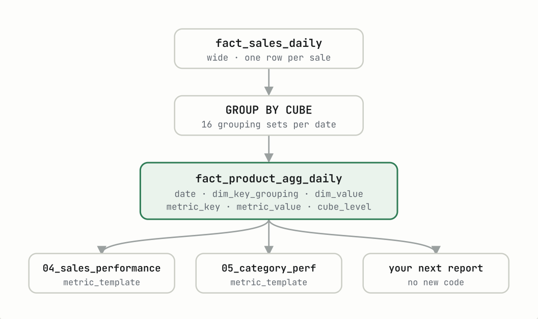
An entire sales pipeline — years of history, four cubed dimensions, dozens of derived metrics — can land in exactly one table shape: date, dim_key, dim_key_grouping, dim_value, metric_key, metric_value, cube_level. There is no revenue column and no wow column. There is a metric name and a metric value.
This is the entity–attribute–value model in the dialect that suits analytics: a long fact table rather than a wide one. Narrow tables absorb new fields without touching the schema; wide ones make cross-metric arithmetic easier. But the shape alone isn't what makes this a reporting substrate — the two addressing conventions layered on top are.
What's used in the blog
The pipeline is dbt_sales_reporting, a seven-task workflow in the LeastAction catalog. Five catalog item types carry the pattern.
Pipeline · dbt_sales_reporting
What it is: the workflow the report tasks belong to — a seed, three dbt stages, a validation task, and two report tasks.
What it is used for here: it produces fact_product_agg_daily, the key–value table every report reads.
Operator · PostgresqlGenerateHtmlTableReport
What it is: an operator is the code a task runs. This one reads the key–value fact table, pivots it according to the payload, renders an HTML table, writes it to a Postgres output table, and posts it to the catalog as an html_report asset.
What it is used for here: both report tasks — 04_sales_performance_report and 05_category_performance_report — point at this same operator. Nothing about either report is expressed in code; the difference between them is the payload.
Connection · dbt_postgresql
What it is: a connection holds the credentials and host for a system a task talks to.
What it is used for here: connection.postgresql pointing at postgres-demo:5432/postgres_demo_db, the warehouse holding fact_product_agg_daily. The dbt model tasks and both report tasks share it.
Payload · the report, as data
What it is: a payload is the JSON, text or sql a task passes to its operator at runtime.
What it is used for here: data, holding report_title, output_table, output_parent_laui, report_style, date_columns, trend_weeks, summary_columns, query, and metric_template. This is what differs between the two reports.
{
  "data": {
    "report_title": "Sales Performance Dashboard",
    "date_columns": 4,
    "summary_columns": ["trend", "std", "yoy", "share"],
    "query": { "table": "fact_product_agg_daily" },
    "metric_template": [
      {
        "display_name":     "Revenue by Region",
        "dim_key_grouping": "dim_product::dim_category::*::dim_subregion",
        "metric_key":       "revenue",
        "cell_format":      "${value:,.0f}"
      }
    ]
  }
}
Actions · pre_action and post_action
What it is: an action is a hook that can be attached to a task's lifecycle which the platform fires/invokes.
What it is used for here:
- pre_action —
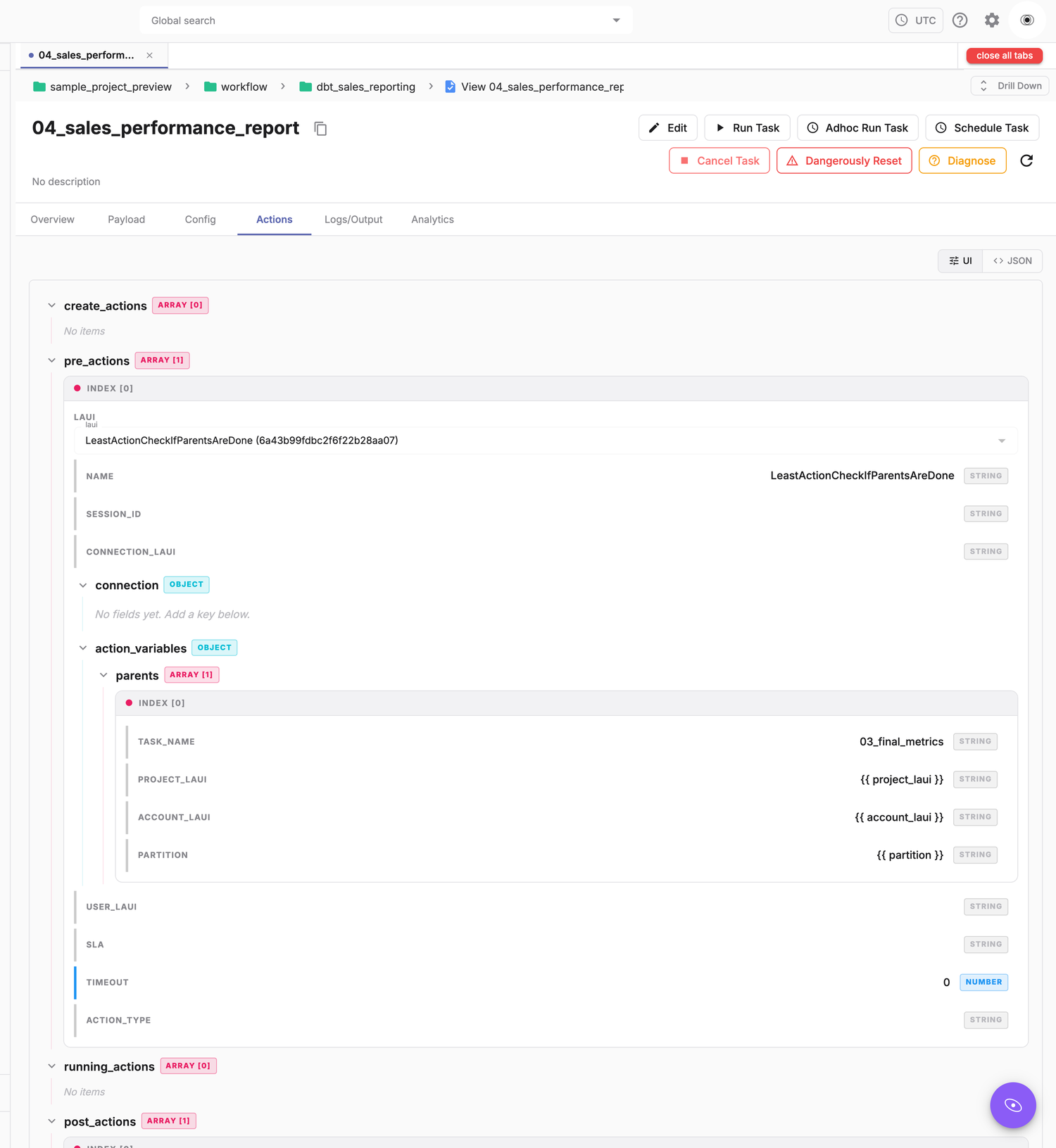
LeastActionCheckIfParentsAreDone, listing03_final_metricsas its parent. The report waits for that task to reach success, so it cannot render against a half-built table. - post_action —
LeastActionAgentDebug, reading theDBT_Postgresql_Sales_Pipelines_SkillandDBT_Postgresql_Sales_Data_Contractskills.
Convention 1 · Dimension addressing — dim_key_grouping
The naive way to say "revenue, aggregated across all regions" is to leave the region column NULL — but NULL means both rolled up and missing, and you can't pattern-match on it. So a UDF coalesces every rolled-up position to a sentinel instead: COALESCE(p_region, 'dim_region'). A position holding a real value is a filter; a position holding dim_* is rolled up. Every rollup level is now an addressable string with a fixed positional grammar.
Watch it happen on one sale. Ascend Desk Compact / Furniture / Asia Pacific / East Asia goes into the CUBE and comes out as several rows — one per rollup level. Each row runs through both UDFs: generate_dim_key_grouping() fills every rolled-up slot with its sentinel, and generate_dim_value() keeps only the slots that survived.
| Dimensions that survived | dim_key_grouping (the address) | dim_value (the label) |
|---|---|---|
| all four · cube_level 0 | Ascend Desk Compact::Furniture::Asia Pacific::East Asia | Ascend Desk Compact::Furniture::Asia Pacific::East Asia |
| no category · cube_level 1 | Ascend Desk Compact::dim_category::Asia Pacific::East Asia | Ascend Desk Compact::Asia Pacific::East Asia |
| product + region · cube_level 2 | Ascend Desk Compact::dim_category::Asia Pacific::dim_subregion | Ascend Desk Compact::Asia Pacific |
| product only · cube_level 3 | Ascend Desk Compact::dim_category::dim_region::dim_subregion | Ascend Desk Compact |
| none — grand total · cube_level 4 | dim_product::dim_category::dim_region::dim_subregion | (empty string) |
Row three is why the two columns can't be one column. Its label reads Ascend Desk Compact::Asia Pacific, which has lost the fact that those were the first and third slots — fine for printing, useless for matching. The address keeps the positions; the label throws them away. The grand total's label is the empty string, which is how the renderer finds it when it needs a denominator.
Filtering is then just pattern-matching that address. Each slot in a template means one of three things:
| You write | It matches |
|---|---|
Ascend Desk Compact | Only that literal value in that slot. A filter. |
dim_region | Only rows where region was rolled up. Also a literal — the sentinel is just text. |
* | Any real value, and you get one report row per distinct value found. |
So dim_product::dim_category::*::dim_subregion reads as: every product, every category, one row per region, sub-regions rolled up. The operator turns that into a regex — twice, and not the same regex:
# pushed down to Postgres — deliberately loose, a memory guard
'^dim_product::dim_category::[^:]+::dim_subregion$'

# applied again in pandas — the strict one
'^dim_product::dim_category::(?!dim_)[^:]+::dim_subregion$'
The difference is (?!dim_). Without it, [^:]+ matches the literal text dim_region, so the loose version also returns the rows where region was rolled up, which would appear as an extra row alongside the real regions.
Convention 2 · Metric addressing — metric_key
Derived metrics are the same metric with a suffix, never a new column: _dod, _wow, _avg_10d, _std_10d, _ytd, _yoy, _rank, _pct_of_total. Each is a UNION ALL block that reads the previous stage and re-emits rows with a mangled key.
One address, one base measurement, and the models derive the rest around it. Every row below shares the same date and dim_key_grouping — only the key changes.
metric_key | metric_value | Emitted by |
|---|---|---|
revenue | 1000.00 | stage1 — the base CUBE |
revenue_dod | +120.00 | stage2 — 1-row lag |
revenue_wow | −45.00 | stage2 — 7-row lag |
revenue_avg_10d | 940.00 | stage2 — rolling window |
revenue_std_10d | 86.40 | stage2 — rolling window |
revenue_yoy | +310.00 | final — 365-row lag |
The machinery producing one of those rows is the _wow block in full:
with metric_with_lag as (
    select date, dim_key, dim_key_grouping, dim_value, metric_key, metric_value,
        lag(metric_value, 7) over (
            partition by dim_key_grouping, dim_value, metric_key
            order by date
        ) as prev_week_value
    from fact_product_agg_daily_stage1
)
select date, dim_key, dim_key_grouping, dim_value,
    metric_key || '_wow' as metric_key,
    coalesce(metric_value - prev_week_value, 0) as metric_value,
    null::int as cube_level
from metric_with_lag
where prev_week_value is not null
Note null::int as cube_level — derived rows carry no cube level. They aren't a fresh aggregation of the source; they're arithmetic on rows that already exist.
Where it sits
The seven tasks run in order: a seed loads fact_sales_daily, three dbt stages build the cube, a validation task checks the result, and the two report tasks render off the end of it. The report tasks are the last two rows, and they are the only two that read the key–value table rather than writing to it.
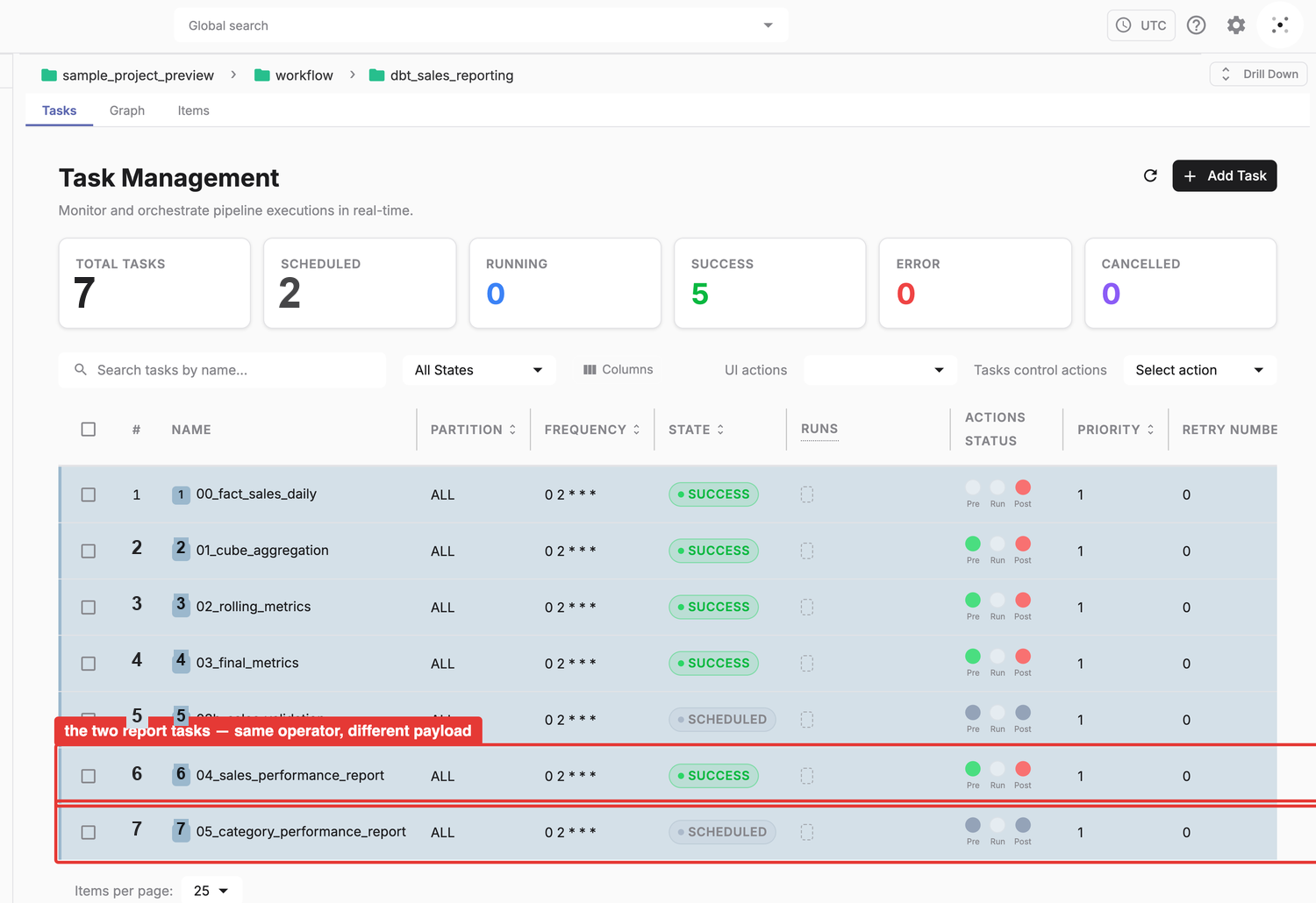
On the run captured here, the seed loaded 404,750 rows. stage1 came out at 10,984,410 rows, stage2 at 46,094,905, and fact_product_agg_daily at 65,722,719 rows carrying 31 distinct metric_key values across five cube levels — 300 fully-detailed groupings, 740 at level 1, 495 at level 2, 48 at level 3, and the single grand-total row at level 4.
Different cases
We changed one character in one field of the payload, in two directions, to see what the operator does with it. All three blocks name the same metric, read the same table, and run through the same operator. They differ only in how many slots of dim_key_grouping hold a wildcard.
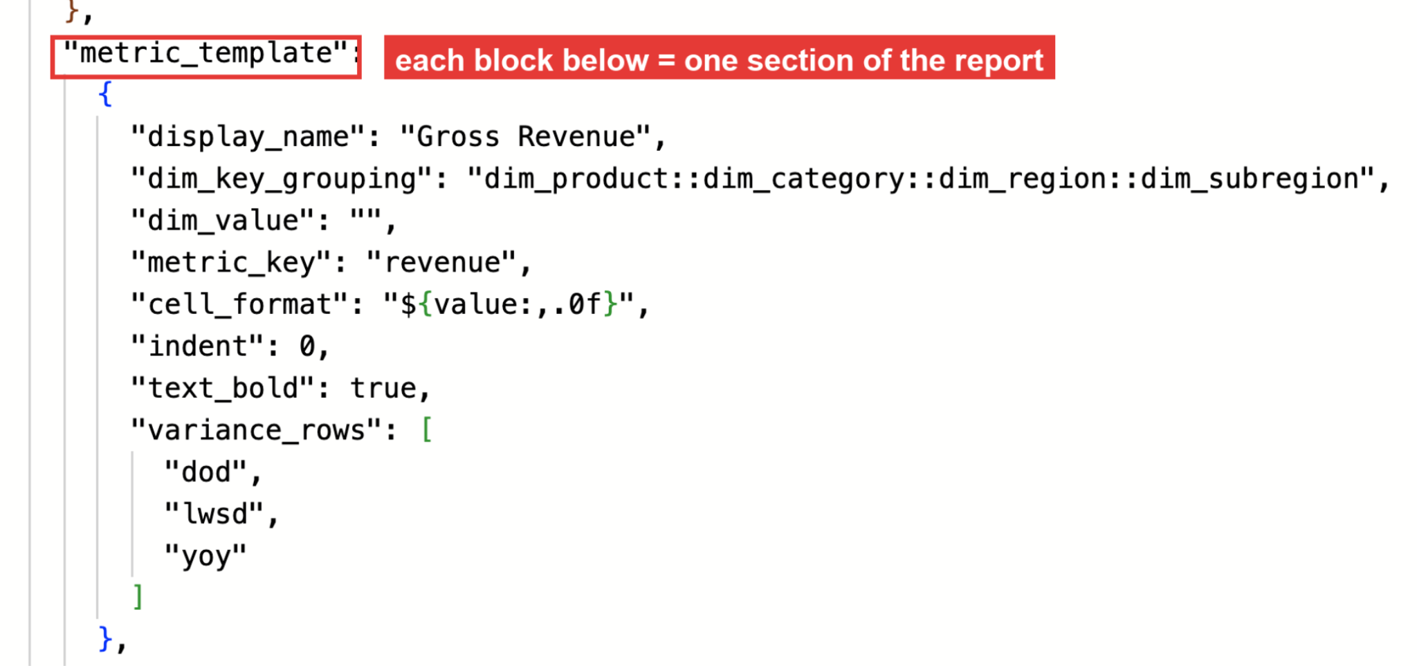
Case 1 · every slot pinned
{
  "display_name":  "Gross Revenue",
  "dim_key_grouping": "dim_product::dim_category::dim_region::dim_subregion",
  "dim_value":     "",
  "metric_key":    "revenue",
  "variance_rows": ["dod", "lwsd", "yoy"]
}
Every position holds a sentinel, so the address matches exactly one row per date — the fully rolled-up row, whose dim_value is the empty string. The report renders a single line, Gross Revenue, with the three variance rows that block asked for indented beneath it.
Case 2 · one slot wildcarded
{
  "display_name":  "Revenue by Product",
  "dim_key_grouping": "*::dim_category::dim_region::dim_subregion",
  "metric_key":    "revenue",
  "sort_order": "value", "limit": 10,
  "variance_rows": ["dod"]
}
The first position becomes *. The same address now matches every row where the product slot holds a real value, and the operator emits one report row per distinct value it finds — ten of them, ordered by value and cut by limit. No product name appears anywhere in the payload; the rows come from what the wildcard found in the table.
Case 3 · two slots wildcarded
{
  "display_name":     "Revenue by Product and Region",
  "dim_key_grouping": "*::dim_category::*::dim_subregion",
  "metric_key":       "revenue",
  "sort_order": "value", "limit": 10
}
The product slot and the region slot become *. The address now matches every row where those two positions each hold a real value, and the operator emits one row per combination it finds — product crossed with region, ordered by value and cut by limit. The wildcards compose: nothing in the operator special-cases one wildcard versus two.
Same operator, same table, same metric key, same run. The output goes from one row, to one row per product, to one row per product-and-region pairing — driven entirely by how many positions hold a wildcard. All three blocks are in the payload of 04_sales_performance_report.
Details of how it actually works
Getting the wildcard to resolve against a 65-million-row table, and the numbers to come out meaning what their names say, took three specific things in the operator.
- The wildcard compiles twice, into two different regexes. A loose form —
*becomes[^:]+— is pushed down to Postgres as adim_key_grouping ~ '…'filter. A strict form —*becomes(?!dim_)[^:]+— is applied again in pandas. The loose one is a superset on purpose: its job is to stop the query returning every grouping in the cube. The strict one excludes rows where that position was rolled up. - Only the metric keys the report needs are pulled. The operator walks the template before querying, collects each block's base
metric_keyplus only the suffixed keys itsvariance_rowsand the report'ssummary_columnsrequire, and pushes that asmetric_key IN (...). A report asking for revenue with a YoY column reads two keys out of the 31 in the table. - The share column does not use the cube's own percentage.
revenue_pct_of_totalis computed within a grouping, so on a detail row it is always 100%. For the share summary column the renderer instead locates the fully rolled-up row — the one whosedim_valueis the empty string — and divides by that.
Know the edges
- Everything is stringly-typed.
metric_keyis a TEXT column. Ship a model that emitsrevenue_WoWand nothing fails — the report is just silently empty. A validation gate asserting a floor on distinct metric keys and no NULL values reports the symptom after the load rather than the typo at the point it was written. A metric-key registry checked in CI catches the typo at commit time instead. - Memory is the real failure mode. The unrestricted version of the report query returns every grouping in the cube over the whole window and exhausts the worker's memory. The operator pushes a coarse grouping regex and a narrow
metric_key IN (...)list down to the database, then filters precisely in memory. - Cardinality needs governing. A CUBE with one dimension too many multiplies the whole table by that dimension's cardinality. This repo ships a
dim_cube_config.csvwith aninclude_in_cubeflag per dimension, but nothing reads it — the list is hardcoded in the model'scube(...)call. Flipping the flag changes nothing. The field reads as a control, so a change made there can be expected to take effect when it does not. - A metric name is not a metric definition.
revenue_pct_of_totalis computed within a grouping, so for a detail row it is always 100%. Correct by its own definition, and not what "share of business" means. The name and the meaning can drift apart, and nothing here catches it. - It costs storage, and most of the storage is derived rows. On the run captured here, 404,750 source rows in an 82 MB table became 65,722,719 rows in a 13 GB table — a factor of 162, before counting the two intermediate stages. Inside that final table, 16.7% of the rows are base CUBE output and 83.3% are derived rows carrying the suffixed keys, so five-sixths of the volume is arithmetic over the other sixth. Rebuild cost tracks the same shape: every run recomputes all of it.
| Table | Rows | On disk |
|---|---|---|
fact_sales_daily — source | 404,750 | 82 MB |
| stage1 — the CUBE | 10,984,410 | 2,182 MB |
| stage2 — rolling metrics | 46,094,905 | 9,244 MB |
fact_product_agg_daily — final | 65,722,719 | 13 GB |
Comparison
There are many methods of doing metric standardization, here is a comparison with SSAS, which can be used in the same way using MDX queries.
| SQL Based Cube | SSAS | |
|---|---|---|
| Metrics based on | SQL in dbt models. A metric is a row (metric_key / metric_value). Portable to any SQL warehouse. | A cube model. Measures and calculated members in MDX (Multidimensional) or DAX (Tabular). |
| Hosting | Nothing beyond the warehouse already in use. Tables sit in Postgres next to the source. | A separate SSAS instance to install, license and operate. |
| Efficiency | Lookup — the aggregation already ran. Any rollup level costs the same. | High. Server caches and serves from stored aggregations. |
| Build / storage cost | The main cost. Measured here: 404,750 rows / 82 MB → 65.7M rows / 13 GB, a factor of 162. Every run rebuilds all of it. | Moderate. Materialises a chosen subset of aggregations, tuned against usage. |
| Standardization | High. Every metric is a materialized row under one naming convention; the vocabulary is enumerable via SELECT DISTINCT metric_key. | Medium. Definitions are central to the cube, but consumers write MDX/DAX to reach them. |
| Adding a metric | One UNION ALL block, rebuild the models. No schema change, no consumer notice. | Add a calculated member, reprocess the cube. |
How to Set Up in LeastAction
This is the walkthrough for the report task described above. It assumes the key–value table already exists — the dbt stages that build it are a separate piece of work. What follows is only the reporting layer on top of it.
Prerequisites
- A table in the key–value shape:
date,dim_key,dim_key_grouping,dim_value,metric_key,metric_value,cube_level. Here that isfact_product_agg_daily, built by the three dbt tasks. - A Postgres connection in the catalog pointing at that warehouse —
dbt_postgresqlin this project. - The
PostgresqlGenerateHtmlTableReportoperator in your catalog, under operator → Postgresql. - A folder to publish into. This project uses an asset folder called
sales_pipeline_reports; its LAUI goes in the payload asoutput_parent_laui.
Step 1 — point a task at the operator and the connection
Create a task in the workflow folder, select PostgresqlGenerateHtmlTableReport as the operator and dbt_postgresql as the connection. This pair is identical for every report built this way; only the payload in step 2 changes.
Step 2 — write the report as the payload
The Payload tab holds the JSON. query.table names the key–value table. date_columns sets how many date columns are rendered and trend_weeks how far back the trend is computed. summary_columns lists the analytic columns on the right. metric_template is the report body: one block per section.
Step 3 — gate it on the table it reads
On the Actions tab, add LeastActionCheckIfParentsAreDone as a pre_action and list the task that builds the table — here 03_final_metrics. The report then waits for that task to reach success before it runs, so it cannot render against a partially built table.
How to Use in LeastAction
LeastAction comes prebuilt with all the tasks, so setup will not be needed in this case, all you will need to do is follow the below 2 steps after installation.
Step 1 — run the task
Run the task from the task page, or leave it on its schedule. The pre_action holds it until 03_final_metrics reports success, then the operator queries the key–value table, renders the HTML, writes it to the output table, and posts it to the catalog folder named in output_parent_laui.
Step 2 — read the result in the catalog
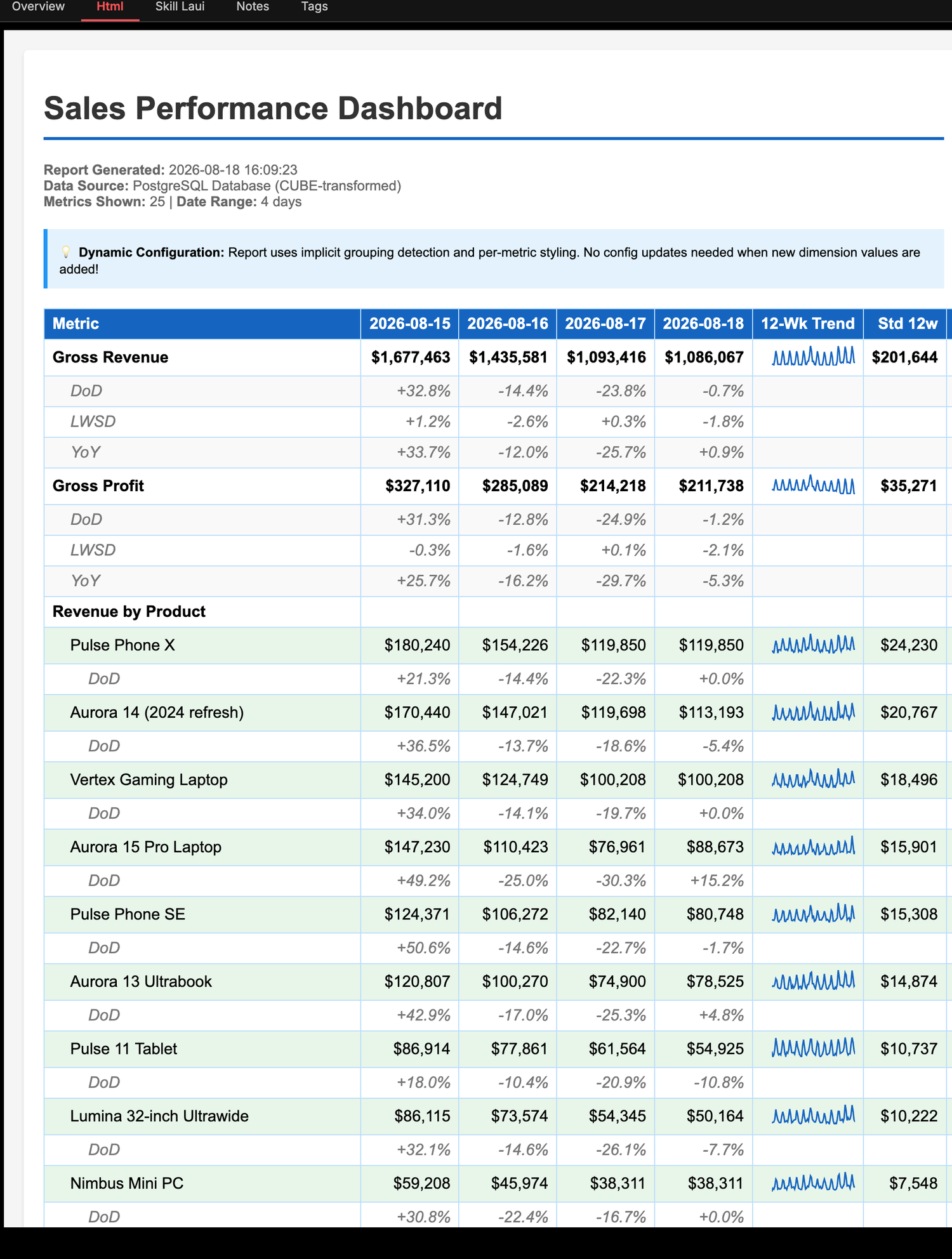
The report appears in the asset folder as an html_report item, timestamped, with the rendered table on its Html tab. The run captured here produced 25 rows across 4 date columns.
The rendered output maps back to the payload one block at a time. Gross Revenue and Gross Profit are the two grand-total blocks, each followed by its indented DoD, LWSD and YoY rows. 12-Wk Trend and Std 12w are the first two entries of summary_columns, the trend drawn as an inline SVG sparkline.
Comments (0)
to join the conversation.
No comments yet — be the first to say something.